“The attempt to combine wisdom and power has only rarely been successful and then only for a short while.” Albert Einstein
I figure I best write down my thoughts before my new found wisdom escapes me. Every time I think I’ve finally understood “Filter Context”, it turns out that I really don’t get it.
To be honest, I’ve read many definitions of “Filter Context” and descriptions about “Filter Context”. None of them have helped me to master the concept. I don’t come from the world of the multi-dimensional language MDX. Until recently, I didn’t see the usefulness of PivotTables when a solid SQL query can provide the same information.
Then, it came to me! What if I used the knowledge that I do have? Look at PivotTables and “Filter Context” through the perspective of SQL. Using this new perspective, I believe “Filter Context” is the following:
the key concept in PowerPivot allowing you to use Excel-like functions to dynamically alter the criteria of each cell in a PivotTable. Instead of relying on the PivotTable’s built-in process of creating a criteria based on the row value, column value, report filter, and/or slicer, utilize DAX functions to define the criteria. This new capability removes the PivotTable’s limited ability to solve business problems.
You can now move beyond the standard SUM and COUNT formulas, and create functions similar to those in SQL. “Filter Context” isn’t a feature like something you can select in an Excel ribbon or pop-up menu. It’s a behavior similar to Excel’s cell reference. Once you understand for example what the cell reference “A1:C3” is, you can use it in all sorts of Excel functions. Just like cell reference, “Filter Context” is fundamental to creating DAX formulas.
I took my thoughts a little further. How does a PivotTable operate? It executes a SQL statement in each cell. Those SQL statements’ “where” clauses are automatically created based on the cell’s position in the PivotTable.
Let me start with a very basic data-set (call it data_table),
ID
|
Product
|
Color
|
amount
|
1
|
Pen
|
Red
|
2
|
3
|
Pencil
|
Blue
|
6
|
5
|
Pen
|
Blue
|
10
|
7
|
Pencil
|
Red
|
10
|
Create a standard PivotTable from the above data table,
I create the PivotTable below by:
· Dragging Color into Row labels
· Dragging Name into Column labels
· Dragging amount into Values and leaving the “Summarize values as” SUM function
· No Slicer or PivotTable’s report filter was used
You get something like below,
Sum of amount
|
Column Labels
| |
Row Labels
|
Pen
|
Pencil
|
Blue
|
10
|
6
|
Red
|
2
|
10
|
Not too useful!
If I apply my SQL analogy, the PivotTable really looks like,
Column Label (Product)
| |||
Row Label (Color)
|
Pen
|
Pencil
| |
Blue
|
select sum(amount)
from data_table where Color = 'Blue' and Product = 'Pen' |
select sum(amount)
from data_table where Color = 'Blue' and Product = 'Pencil' | |
Red
|
select sum(amount)
from data_table where Color = 'Red' and Product = 'Pen' |
select sum(amount)
from data_table where Color = 'Red' and Product = 'Pencil' | |
Each of the 4 cells in my PivotTable execute a query off of my data_table. In the cell that intersects Pen and Blue, SUM(amount) function will execute only for rows in the data_table where Color = 'Blue' and Product = 'Pen'. No matter where I place this PivotTable in my worksheet or the entire workbook, this cell will always execute the SUM(amount) function where Color = 'Blue' and Product = 'Pen'.
What’s the big deal?
The standard PivotTable executes the SQL statements each time you refresh the table or alter the criteria of PivotTable. Basically, the PivotTable dynamically creates the “where” clause criteria based on the location of the SQL statement inside the PivotTable. The only way to alter this SQL statement is select a different aggregation function (COUNT, AVERAGE, and MAX). Not very flexible or useful for healthcare analytics!
In order to make a useful function, say a ratio of amount of Blue Pens to all Pens and Pencils, a PowerPivot function needs to be created. More appropriately, a DAX function needs to be created. PowerPivot allows you to create your own “where” clause statement, even join multiple tables, or utilize functions other than COUNT, AVERAGE, and MAX. This fact turns Excel’s PivotTable into a true Business Intelligence tool.
EXAMPLE DAX FORMULA #1 - Create a formula to compute Total Amount of all Pens and Pencils
In terms of SQL, I need to create a “where” clause that ignores both the row label and column label criteria for each cell of the PivotTable. That would look like,
Column Label (Product)
| |||
Row Label (Color)
|
Pen
|
Pencil
| |
Blue
|
select sum(amount)
from data_table where (ignore Color = 'Blue' and ignore Product = 'Pen') |
select sum(amount)
from data_table where (ignore Color = 'Blue' and ignore Product = 'Pencil') | |
Red
|
select sum(amount)
from data_table where (ignore Color = 'Red' and ignore Product = 'Pen') |
select sum(amount)
from data_table where (ignore Color = 'Red' and ignore Product = 'Pencil') |
That is, I want my PivotTable to ignore the built-in “where” clause of “where Color = 'Blue' and Product = 'Pen'” and utilize a “where” clause of my creation. I want the total of all Pens and Pencils to appear in each cell of my PivotTable.
To ignore the PivotTable’s built-in where clause statement, I created the following DAX formula,
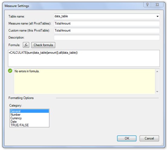
TotalAmount=CALCULATE(sum(data_table[amount]),all(data_table))
This is analogous to writing,
SELECT sum(data_table[amount])
FROM data_table
I want to compute the total amount regardless of where this function is placed in the PivotTable. I don’t care if the end user slices the PivotTable by Red and dices the PivotTable by Pen resulting in only one cell in the PivotTable, I want to override the PivotTable’s built-in criteria. The SQL statement is a simple one, sum all values in the column [amount] in the table data_table.
Let’s look at the DAX formula (called a measure in PowerPivot terminology) again,
TotalAmount=CALCULATE(sum(data_table[amount]),all(data_table))
DAX function breakdown
· TotalAmount – name of the measure
The formula that changes the criteria (changes the “filter context”). In my example, CALCULATE sums all the amounts in the table regardless of its position in the PivotTable or criteria selected by the user.
o <expression> -
§ sum(data_table[amount]) – simple formula to sum the amounts in the data_table
o <filter1> -
§ all(data_table) – return all the rows in data_table regardless of the cell this formula is located.
In the PowerPivot’s Field list, right click on the table and select new measure. Excel exposes the dialog box below for you to enter your DAX function,
By selecting the TotalAmount measure only, the PivotTable looks like,
TotalAmount
|
Column Labels
| |
Row Labels
|
Pen
|
Pencil
|
Blue
|
28
|
28
|
Red
|
28
|
28
|
If I include the sum of amounts and TotalAmount measures, the PowerPivot table looks like,
Column Labels
| ||||
Pen
|
Pencil
| |||
Row Labels
|
Sum of amount
|
TotalAmount
|
Sum of amount
|
TotalAmount
|
Blue
|
10
|
28
|
6
|
28
|
Red
|
2
|
28
|
10
|
28
|
EXAMPLE DAX FORMULA #2 - rank the 4 items in the data table by amount
I want to rank the each row of data_table by each row’s amount. In SQL, I would write (using T-SQL):
SELECT ID, amount, RANK() OVER (ORDER BY amount) as Rank
FROM data_table
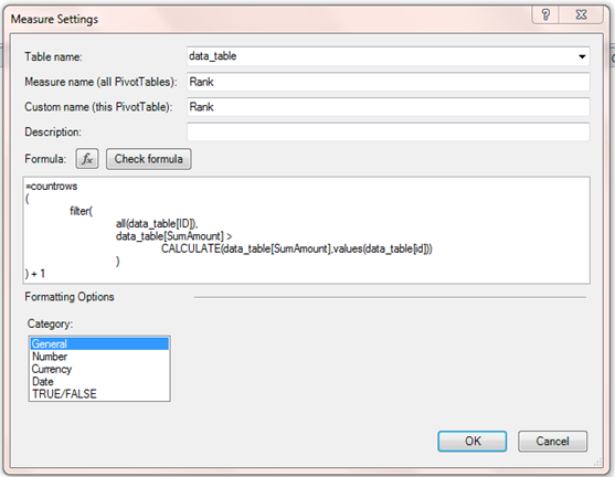
Leave it to Microsoft to provide multiple ways to calculate rank in DAX. I’m choosing to review a longer version for demonstration purposes (PowerPivot version 2 has a built-in RANK function),
Rank=COUNTROWS
(
FILTER(
ALL(data_table[ID]),
data_table[SumAmount] >
CALCULATE(data_table[SumAmount],values(data_table[id]))
)
) + 1
DAX function breakdown
· COUNTROWS(<table>) – Count the number of rows in the table defined by formulas defined inside the parenthesis
· FILTER(<table>,<filter>) - Returns a table to the COUNTROWS function that only contains rows that have amounts greater than the row that this function is located.
o First, ignore the row and column criteria in each cell
o Then compute the ranking algorithm,
data_table[SumAmount] > CALCULATE(data_table[SumAmount],VALUES(data_table[id]))
§ For each row, evaluate whether the current’s rows amount is greater than selected row
§ In order for this formula to work, the measure, data_table[SumAmount] , must be utilized.
· SumAmount =sum(data_table[amount])
The resulting PivotTable looks like,
ID
|
SumAmount
|
Rank
|
1
|
2
|
4
|
3
|
6
|
3
|
5
|
10
|
2
|
7
|
12
|
1
|
PowerPivot allows you to alter the standard PivotTable by:
· Creating powerful, dynamic functions
· Create useful formulas such as pmpm, per 1000, percent compliance
There is a lot of nuance in “Filter Context” that I didn’t describe. I wanted to share my new understanding of the key PowerPivot concept. Key items to remember:
· When a measure is placed in a PivotTable, it’s execution in each cell depends on the intersection of row, column, report filter, and slicers. In essence, PowerPivot allows you to change this intersection by using DAX functions
· Think of “Filter Context” as changing the ”where” clause statement in a SQL statement.
· PowerPivot allows for the creation of useful functions inside PivotTables, similar to functions in a standard Excel worksheet. Percent compliance rates, per member per month, and encounters per 1000 are a few of the metrics that can now be calculated on the fly inside an Excel PivotTable.


No comments:
Post a Comment